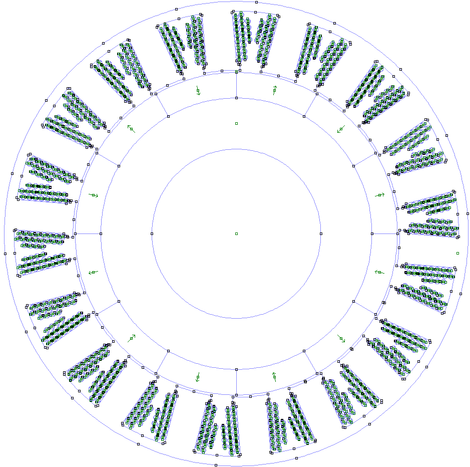
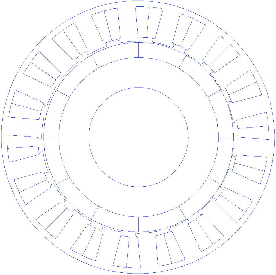
This page talks about the Parameterized Inner Rotating BLDC type Motor with Surface Mounted Permanent Magnets

This type of motor is a standard surface mounted PM BLDC motor, and some variations of it.

Initial Setup

Software setup

Download and install Scilab 5.5.2 and FEMM 4.2. The rlib’s bin files can be obtained from me.

Activate the libraries

The rlib has many functions which are split according to their use, into individual binary files. Loading the binary files also loads the functions into the Scilab’s working memory. Additionally, FEMM provides a set of linking functions that interface Scilab with FEMM through a dll file and corresponding scilab functions.

The common_odr file has functions that are essential to handle the data. The common_motor file has functions that are essential for all motor topologies. The geom_irbldc file has functions that are useful for creating the motor variable and the optimization variable for the irpmbldc topology. In addition, this file also has functions to build the motor model in FEMM from the motor variable.

Script to activate the libraries is below.

exec('D:\femm4.2\scifemm\scifemm.sci', -1);
load('Y:\MOTOR\scripts\r_lib\r_common_odr.bin');
load('Y:\MOTOR\scripts\r_lib\r_common_motor.bin');
load('Y:\MOTOR\scripts\r_lib\r_geom_irbldc.bin'); 

Build the model from the default template

The geometry from the motor variable is checked for any errors and geometrical feasibility. If the motor can not be constructed for any reason, the reason is printed out and the model is not built. Script to build the model with default template is below.

Motor=r_buildMOTOR(12,18) // poles, slots

or alternatively,

Motor=r_buildVAR(12,18) // poles, slots
Motor=r_buildMOTOR(Motor)

The motor variable can be constructed with as little as 2 inputs and as many as 8 inputs.

Motor=r_buildVAR(12,18) // poles, slots
Motor=r_buildVAR(12,18,50) // poles, slots, outer radius
Motor=r_buildVAR(12,18,50,15) // poles, slots, outer radius, stack depth
Motor=r_buildVAR(12,18,50,15,0.5) // poles, slots, outer radius, stack depth, air gap
Motor=r_buildVAR(12,18,50,15,0.5,'STAR') // poles, slots, outer radius, stack depth, air gap, winding type
Motor=r_buildVAR(12,18,50,15,0.5,'STAR',48) // poles, slots, outer radius, stack depth, air gap, winding type, voltage range
Motor=r_buildVAR(12,18,50,15,0.5,'STAR',48,80) // poles, slots, outer radius, stack depth, air gap, winding type, voltage range, current limit
// Each of the above generates a valid motor variable, assuming the default values for rest of the parameters wherever they are not provided. 

Or, the simpler notation as below can be used to specify only those parameters that are of interest, while others are assumed to be same as the in the default template.

Motor=r_buildVAR('poles',12,'slots',18,'throw',2)
Motor=r_buildMOTOR(Motor)
// or 

Motor=r_buildMOTOR('poles',12,'slots',18,'throw',2)

Special calling references: poles/pole, slots/slot, outerrad/rad, outerdia/dia, stacklen/len, airgap/gap, winding/wind/windtype, vdcrated/vdc, idcmax/idc, and coilthrow/throw.

The r_buildMOTOR function call with the same inputs as r_buildVAR will build the motor with the parameters, effectively reducing the command count by 1. Similarly, the r_solve after r_buildVAR will also build the motor.

Configuration

Geometric parameters

Poles and Slots

The poles and slots need to be selected to incorporate a balanced winding pattern. A balanced winding is the one in which all the three phase vectors on the 2-D surface of the motor winding are separated by 120 electrical degrees. Only a few pole slot combinations are valid. The rlib automatically chooses the rest of the parameters such as the tooth width, magnet arc length, etc.

Motor.Rotor.Poles=12
//poles have to be a multiple of 2
Motor.Stator.Slots=18
//slots have to be a multiple of 3

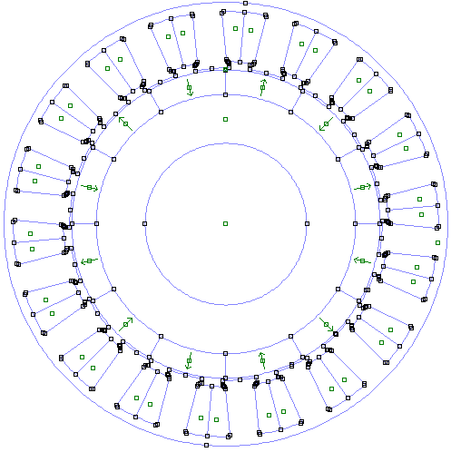
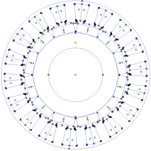
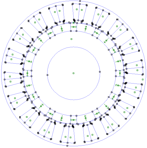
Poles and slots combination alters few other geometric parameters on the stator, rotor as well. A small animation to show the stator changes when the fixed pole rotor is paired with stator with varying slot count.

Outer radius and stack depth

These two are independent parameters and are global values. The rlib chooses rest of the parameters of the motor to fit within the outer_radius parameter. When motor variable is created using the r_buildVAR or r_buildMOTOR, with only the outer radius, the default template will come up with rest of the parameters scaled appropriately to result in a valid motor geometry. The stack depth is the length of the motor in the axial direction. These two parameters can be set with the following script

Motor.Stator.Outer_rad=50
Motor.StackDepth=15

Air gap

Air gap of the motor is the distance between the stator and the rotor when the motor is assembled. The rlib changes the stator geometry and retains the rotor geometry when the air gap is changed, while the template variable is being created. A small animation with the changing air gap is presented below.

Motor.Airgap=0.5

Tooth wedge angle

The tooth wedge angle is the angle of the tooth edge with respect to the line through its center. This angle can be customized in rlib resulting in many possibilities. It is necessary to observe that the toothwedgeangle for ORPMBLDC is opposite in sign to that of this motor type, due to the notation used during the consutrction.

Motor.Stator.ToothWedgeAngle=-5

Magnet PoleArc

Pole arc is the fill of each pole in one electrical angle span. This alue is in the range (0,180]. Script to change the magnet’s pole arc

Motor=r_buildVAR(12,18)
Motor.Winding.Turns=8
Motor.Stator.forcedParallelSlot=1
Motor.Rotor.Polearc=120
Motor=r_buildMOTOR(Motor)

Magnet thickness

Magnet thickness is the thickness of the hard magnetic material in radial direction. Any air gaps between magnets and the back-iron is not assumed. All the magnets are modeled as arc magnetic elements. No chamfer or a fillet addition to the edge is modeled.

Motor.Rotor.Magnet_thickness=5.5

A small animation with changing magnet thickness is presented below.

Stator back iron thickness

Stator back iron is the supporting structure for the stator teeth, and also the conductive path for the magnetic field lines through the stator teeth.

Motor.Stator.BI_thickness=2.1

A small animation with changing back-iron thickness is presented below.

Stator slot depth

Motor.Stator.SlotDepth=20

Slot depth is a measurement taken from the slot bottom point to the edge of air-gap. A small animation showing slot depth variations is presented below. Slot depth can not also change infinitely, because it affects several other parameters such as tooth width etc. too.

Stator slot opening

Motor.Stator.SlotOpening=2

Slot opening is the gap between the consecutive tooth shoe fins in tangential direction. More slot opening lets the winding slip in easily, but increases flux leakage within the stator. A small animation that shows changing slot opening is presented below.

Stator slot open angle

Motor.Stator.SlotOpenAngle=25

The slot opening angle is the angle cast by the line joining stator tooth and the tooth shoe’s inner edge(away from the airgap), with the tangential line at the tooth shoe’s inner edge. An animation showing changing slot opening angle is presented below.

Stator tooth shoe thickness

Motor.Stator.TGD=1.1

Tooth shoe is the construction at the end of the tooth stem towards the air gap, usually wider than the tooth width. A shall animation showing changing tooth shoe thickness is presented below.

Stator tooth width

Motor.Stator.TWS=6.8

Stator tooth width is the width of the tooth towards the airgap. This width may change gradually as we move towards the center of the motor, if the toothwedgeangle is not equal to zero. A small animation showing tooth width changes is presented below.

Stator Slot bottom fillet radius

Motor.Stator.SBfillet_rad=1.1

This is the fillet radius at the bottom of the slot.

Stator Slot opening fillet radius

Motor.Stator.SOfillet_rad=1.1

This is the fillet radius of the slot’s top corner.

Additional Geometric parameters

Magnet overhang

Motor.Rotor.MagnetOverhang=0

This is a parameter that is not used for any electromagnetic calculations, and is purely used for calculating the mass of magnets in the solution parameters.

Forced Parallel Slots

Motor.Stator.forcedParallelSlot=0

This is a parameter that is used to create parallel slots, irrespective of pole & slot combination. This parameter overrides toothwedgeangle and always creates the parallel slots with the required toothwedgeangle.

Topological variations

Halbach motor type 1

This type of motor has radial and lateral magnet arrangement. To achieve this effect, use the following code.

Motor.Rotor.HalBach_type=1
Motor.Rotor.HalBach_fraction=0.25

Halbach motor type 2

This type of motor has inclined and lateral magnet arrangement. To achieve this effect, use the following code.

Motor.Rotor.HalBach_type=2
Motor.Rotor.HalBach_fraction=0.25

Rectangular Magnets

This arrangement will create a realistic representation of the magnet arrangement on the rotor when the rectangular magnets are used. The airgap parameter is used to create shortest distance between the magnets and the stator.To have this construction done, the halback type needs to be set to zero, and the rotor’s polearc needs to be set to 180, else this parameter is reset to 0. To achieve this effect, use the following code.

Motor.Rotor.RectangularMagnet=1
Motor.Rotor.RectangularMagGlueThick=0.05 // has to be at least 0.01 mm 
Motor.Rotor.RectangularMagSpacing=0.05 // has to be at least 0.01 mm

Constructional Parameters

Winding

Motor.Winding.Pattern='ABCABCABCABCABCABC' // calculated automatically. May be overwritten.
Motor.Winding.Type='STAR' // can be of type 'STAR' or 'DELTA'
Motor.Winding.Marking_SLOT_TOOTH='TOOTH' // can be of type 'TOOTH' or 'SLOT'. 
// Tooth winding assumes concentrated winding, and the pattern in Motor.Winding.Pattern refers to how the phase wires are would around individual tooth. Capital letter means that the winding is counter-clockwise when seen from the air gap. 
// When tooth winding pattern is given, a '-' symbol in the Motor.Winding.Pattern indicates a tooth left unwound. Alternate '-' symbols result in a single layer winding. The length of Motor.Winding.Pattern has to be same as the number of slots, for the winding pattern to be valid.
// Slot winding can be used to represent any type of winding, be it concentric, concentrated or distributed, and the pattern in Motor.Winding.Pattern refers to how the phase wires go in or come out of the slots. Capital letter means that the positive current comes out of the screen (positive winding turns). 
// When slot winding pattern is given, a pattern with equal length as the number of slots result in single layer winding. A pattern with length equal to double the slot count result in double layer winding. 
// At the moment, transposed winding is not implemented in the geometry. Winding space for two halves in the double layer winding is divided along the slot depth. 
// Winding pattern is implemented in the geometry from a horizontal line and progresses clockwise (in the direction of the phases)

Motor.Winding.Turns=10
Motor.Winding.NStrands=1
Motor.Winding.PPaths=1
//The above three define how the winding is done. The NStrands and PPaths are used while calculating phase resistances. Winding.Type is used while calculating line resistance. NStrands is also used to plot the total conductors when individual conductors are plotted in the geometry.
Motor.Winding.wire.rectangular=0 
//the above setting is the default. If it is 0, circular cross section of the wire is assumed from the below variable.
Motor.Winding.wireDia=1.016
//If the rectangular property is set to 1, then the following two variables decide the geometry of the wire.
Motor.Winding.wire.len=1
Motor.Winding.wire.wid=2
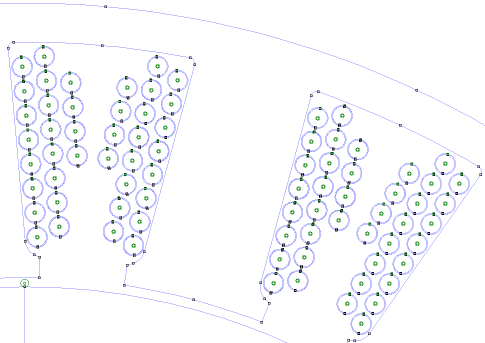
//For representing the individual conductors in the geometry, set the following variable to 1 as shown
Motor.Winding.drawWiresEMag=1
// Wire seperation and insulation thickness of the wires in the geometry can be changed by using the following variables
Motor.Winding.wiregap=0.1
Motor.Winding.insulThickness=0.05
//If resistance estimation is wrong, either because the winding is concentric or distributed type, or because of other reasons, the following variable can be used to force set the resistance to a predetermined value
Motor.Winding.ProjectedRph=0
//Setting the variable to 0 means that the value calculated by rlib is to be used.
//Additionally, a correction factor for the resistance calculation can be included, by the following variable.
Motor.Winding.CorrectionRph=1
//The resistance used in the rlib calculations is the estimated resistance multiplied by the above factor. A value of 1 indicates no change in the estimated resistance.
Motor.Winding.throw=2; // coil throw represented in the number of slot pitches.

//
//

The rlib checks for winding feasibility and generates the winding pattern automatically for the BLDC configuration of single-throw / concentrated winding.

The multi-throw winding will give rise to a configuration in which the slots are split horizontally.

Magnet

Motor.Rotor.MagnetType='Ferrite'

The magnet may be chosen as Ferrite or NdFeB or any other material from the material choice available from the FEMM material library. Magnet’s pole arc can be changed too.

Control parameters

Battery voltage

Motor.Controller.VdcRated=12 // or 48
Motor.Controller.CellsInSeries=1 // or more

This is a very important parameter that decides the maximum speed of the motor. This parameter does not directly decide the operating voltage. This parameter is implemented in two variants of the batteries. When this value is chosen to be less than 15, Lead-Acid is activated. Any value higher than this will indicate Li-ion cells. When the r_buildVAR is used with the Vdcrated parameter, the SoC_V table is automatically populated with the corresponding cell’s Soc vs Voltage and cell resistance value. For a 12 V system, it is assumed that each cell corresponds to 12v nominal voltage. To build a 48v operating voltage, adjust the Motor.Controller.CellsInSeries to 4. For a Li-ion cell system, default number of cells resulting in 48V is 13. Change this number accordingly to adjust the operating voltage. CellsInParallel only effects the pack resistance.

State of Change

Motor.Controller.SoC=50

The state of change for a pack affects the pack voltage as per the SoC_V table. This table is useful for evaluating the performance of the motor at worst case conditions.

Winding temperature

Motor.Winding.TemperatureC=30

The temperature of the winding is a condition that affects the stator resistance seen by the power source, which will reduce the corner rpm on the speed-torque plot for the motor.

Motor Current

Motor.Controller.IdcMax=80
// Forced currents into the winding when solving the model can be set using the following variable. 
Motor.Winding.Cur=[-80 80 0]// These represent the phase currents. in this example, these correspond to star winding currents. 

The IdcMax parameter will set the absolute maximum DC current allowed by the controller. The Cur field in the winding is the current that is passed into the winding for each phase. This cur field is set automatically while solving for the motor model based on the resistance of the winding and the rest of the path, available voltage, and the controller dc current limit. However, a known value may also be given to the model for solving for performance.

Controller resistance

Motor.Controller.Rpath=0.015

The controller path resistance is the PCB resistance that is added to the whole resistance calculation. The complete resistance faced by the available battery voltage decides the corner rpm and the maximum current that the motor can accept for a given voltage.

Material parameters

The field Motor.Prop has all the custom materials defined with their properties. Any materials specified for the magnets from the materials library will assume default values.

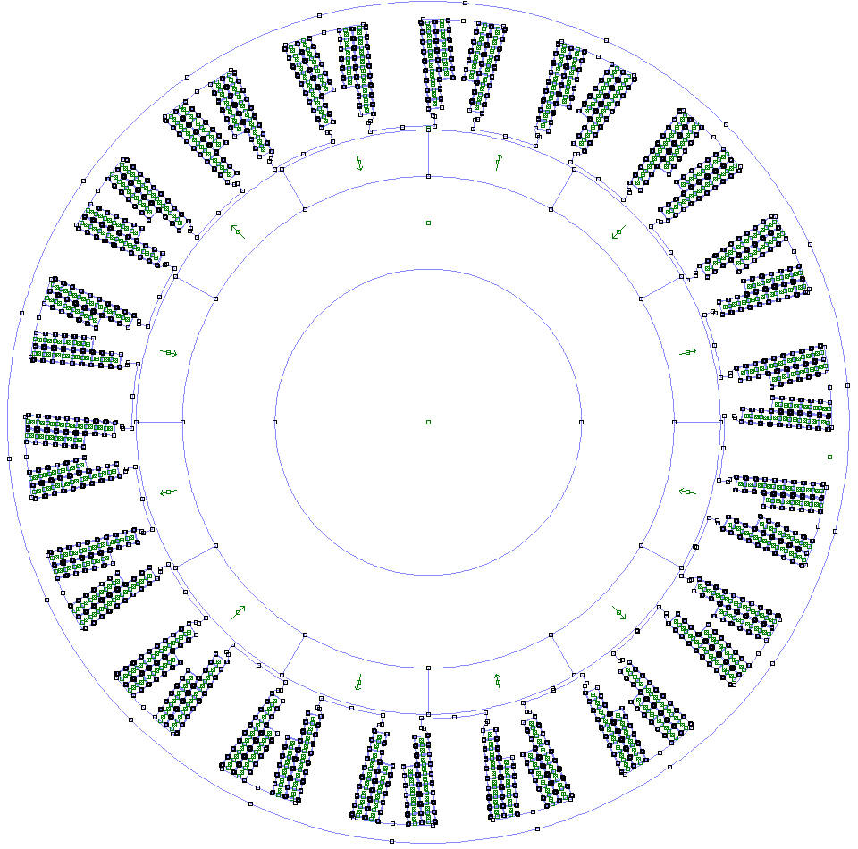
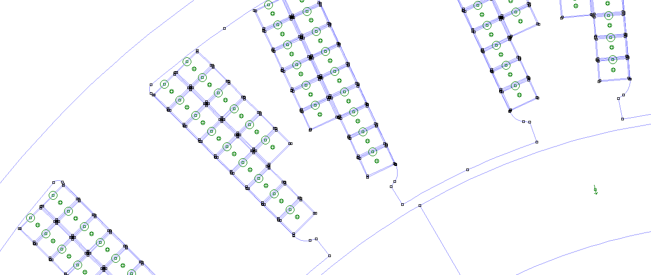
Wire placement

Circular conductors

Script to create the model with individual circular conductors

Motor=r_buildVAR(12,18)
Motor.Winding.drawWiresEMag=1
Motor=r_buildMOTOR(Motor)

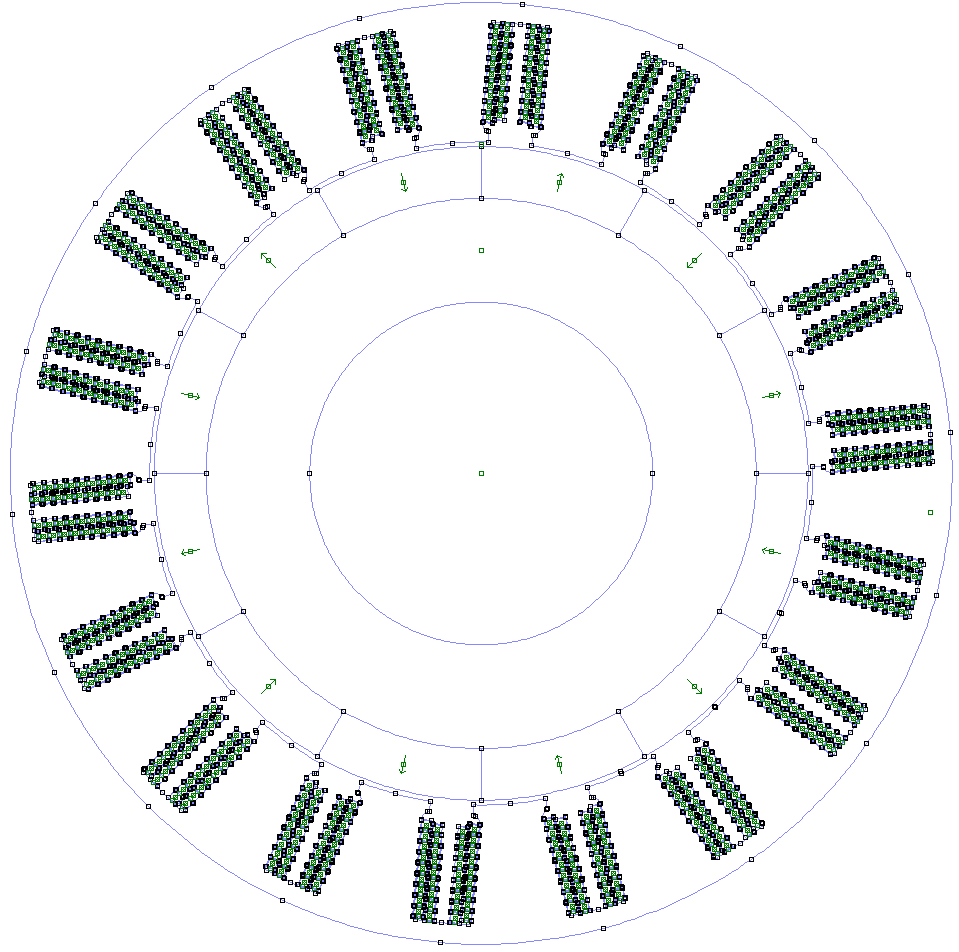
Rectangular conductors

Script to create the model with individual rectangular conductors

Motor=r_buildVAR(12,18)
Motor.Winding.drawWiresEMag=1
Motor.Winding.wire.rectangular=1
Motor.Winding.wire.wid=1.5
Motor.Winding.Turns=8
Motor=r_buildMOTOR(Motor)

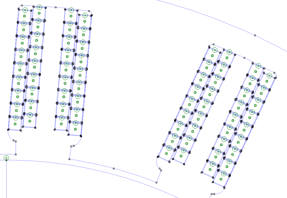
Parallel slots

Script to create parallel slots, instead of parallel tooth, with rectangular conductors

Motor=r_buildVAR(12,18)
Motor.Winding.drawWiresEMag=1
Motor.Winding.wire.rectangular=1
Motor.Winding.wire.wid=3
Motor.Winding.Turns=8
Motor.Stator.forcedParallelSlot=1
Motor=r_buildMOTOR(Motor)

Fault Simulation

Rotor assembly - radial offset emulation

Script to re-create the assembly failure - rotor offset in radial direction

Motor=r_buildVAR(12,18)
Motor.Rotor.Offset.x=0.25
Motor.Rotor.Offset.y=0
Motor=r_buildMOTOR(Motor)

Motor.Rotor.Offset.RotateAboutNewOrigin

The above variable can let us select the type of offset - static (the offset that does not rotate when the rotor rotates) when set to 1, and dynamic (the offset that rotates around along with the rotor) when set to 0.

Running the FEA

Finding the solution

Motor=r_solve(Motor)
Motor=r_solve(Motor,[0,0,0])

The above command will solve the motor based on the current constraints and the voltage input provided in Motor.Controller.

FEMM gives pretty standard outputs for B, H, J across the cross-sectional area.

This function requires a motor structure as an input and optional phase currents [i1,i2,i3] to solve using FEA. If the phase currents are not provided, the geometry is used to calculate resistance, and the controller settings are used to calculate the currents in each phase.

This functions requires the FEMM model to have been created.

This function returns a motor structure with OUTPUT values updated based on the solution. Then the Motor.RUN.dAngle_md is set to non zero values (or when Motor.Solve.ToOUTPUT’s torque line has no starting and ending and incrementa angles), the perturbation is not done to calculate the kb and NLrpm.

The torque after rotating by the angle Motor.RUN.dAngle_md is calculated, along with few other parameters.

OUTPUT is populated based on Motor.Solve.ToOUTPUT parameters.

The syntax is B/H: name,starting radius, ending radius, number of points between radii(including), number of points on each circle, B/H.

fill factor, slot area: name, x coordinate, y coordinate,,,fill/area.

circuit properties, volume, i2r: CircProp/volume/i2r,,,,,circprop/volume/i2r.

Torque: Torq,startAngle,EndAngle,IncrementalAngle,,torque.

When the start/end/increments are given as empty, instantanious fea is done for the single rotor position. When the Motor.RUN.dAngle_md is given to be other than 0, rotor is rotated to that position and solved once.

To solve for no load speed, backenmf constant, keep the torque fields active, and provide a zero Motor.RUN.dAngle_md. Once solved, the rotor is placed at initial position.

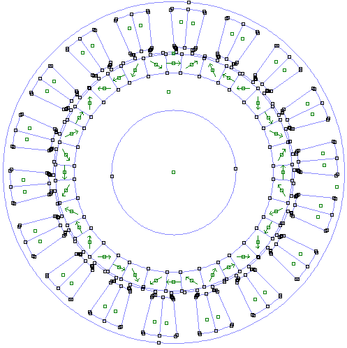
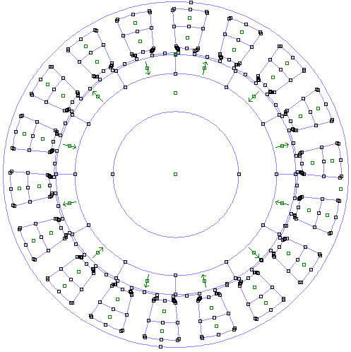
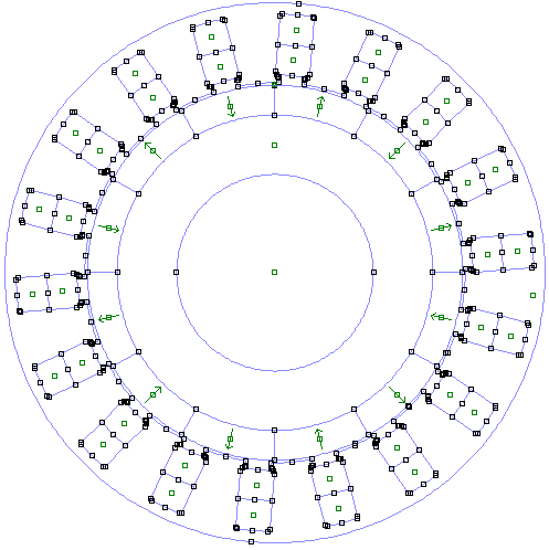
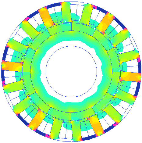
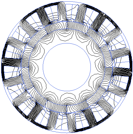
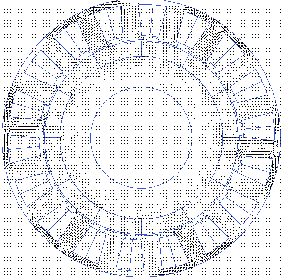
FEMM’s built-in graphical plots

Magnetic flux density (B field)

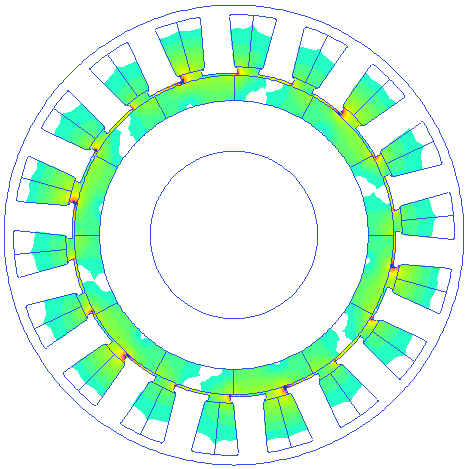
Magnetic field strength (H Field)

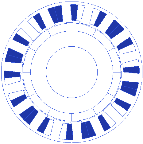
Current density distribution

Iso field lines distribution

Arrow plot for B field

Quantified parameters - with rlib

In addition to the default plots from the FEMM, rlib calculates and plots additional parameters and provides them for the optimization routine.

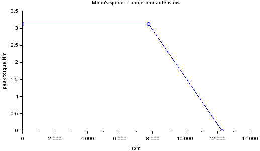
Speed- Torque characteristics

plot(Motor.OUTPUT.rpm_Nm(:,1),Motor.OUTPUT.rpm_Nm(:,2),'.-o')
xlabel('rpm')
ylabel('peak torque Nm')
title('Motor''s speed - torque characteristics')
x=gca()
x.box='off'

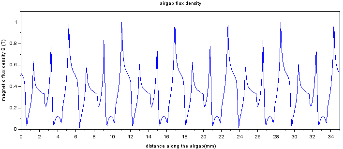
Airgap flux density

x=(0:499)*Motor.Points.rad_airgap/500
a=Motor.OUTPUT.Bgap
plot(x,a)
xlabel('distance along the airgap(mm)')
ylabel('magnetic flux density B (T)')
title('airgap flux density')

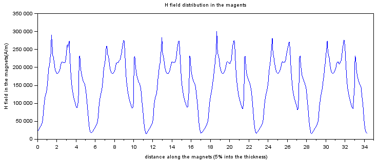
H field inside the magnets

x=(0:499)/500;x=x*(Motor.Stator.Outer_rad-Motor.Stator.BI_thickness- Motor.Stator.SlotDepth- Motor.Airgap - Motor.Rotor.Magnet_thickness*0.05)
plot(x,Motor.OUTPUT.Hmag)
xlabel('distance along the magnets (5% into the thickness)')
ylabel('H field in the magnets(A/m)')
title('H field distribution in the magents')

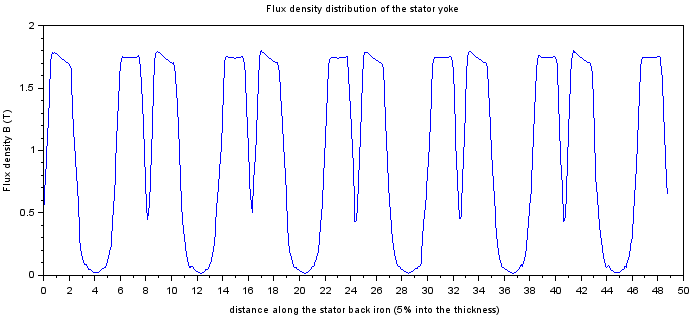
Stator backiron satiration

x=(0:499)/500;x=x*(Motor.Stator.Outer_rad-Motor.Stator.BI_thickness*0.5)
plot(x,Motor.OUTPUT.Bbi)
xlabel('distance along the back iron (5% into the thickness, towards the magnets)')
ylabel('magnetic flux density B (T)')
title('Back iron flux density distribution')

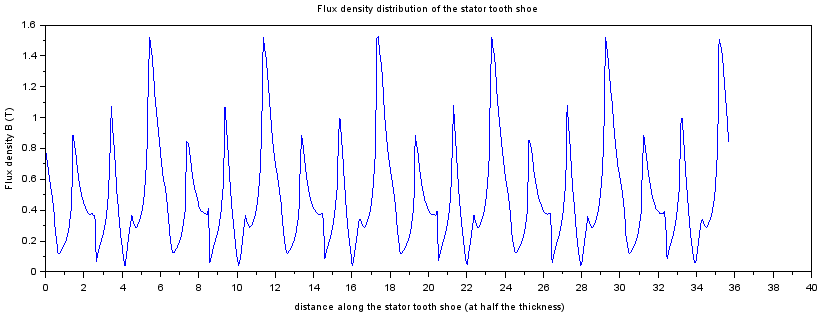
Stator teeth shoe saturation

x=(0:499)/500;x=x*((mydiag(Motor.Points.toothfinouter.x,Motor.Points.toothfinouter.y) + mydiag(Motor.Points.toothfininner.x,Motor.Points.toothfininner.y))/2)
plot(x,Motor.OUTPUT.Bcore.fins)
xlabel('distance along the stator tooth shoe (at half the thickness)')
ylabel('Flux density B (T)')
title('Flux density distribution of the stator tooth shoe')

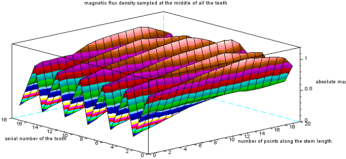
Stator teeth stem saturation

surf(Motor.OUTPUT.Bcore.teeth,'facecol','interp')
xlabel('number of points along the stem length')
ylabel('serial number of the tooth')
zlabel('absolute magnetic flux density')
title('magnetic flux density sampled at the middle of all the teeth')

OUTPUT quantities

Torque

The following stores the peak or instantaneous torque value

Motor.OUTPUT.Torq

The following stores the average torque value, for non-instantaneous solves

Motor.OUTPUT.TorqAvg

The following stores the cogging torque value, for non-instantaneous solves

Motor.OUTPUT.TorqCogging

The following stores the average torque value, for non-instantaneous solves and full solves

Motor.OUTPUT.TorqAvg

RPM

The following stores the maximum rpm of the machine

Motor.OUTPUT.nlRPM

The following stores the corner rpm of the machine

Motor.OUTPUT.CornerRPM

Corner RPM of the machine is that rpm at which the motor’s back-emf becomes sufficient to limit the current into the motor at exactly the controller’s current limit. Any increase in the motor’s rpm will reduce the current into the motor below the controller’s threshold, effectively reducing the torque production.

Back-emf constant

The following gives the back-emf constant

Motor.OUTPUT.kb

Resistance

The resistance of the motor is calculated from the expected copper length and its effective cross section. The effective copper length is calculated including the end-winding length, by considering the average path length for the winding. Any of the following two commands will give the phase resistance.

r1_findrPhase(Motor)

Motor.OUTPUT.Rph

The following will give the line-line resistance

Motor.OUTPUT.Rll

Operating voltage & currents

The following gives the operating battery voltage

Motor.OUTPUT.BAT.voltage

The following gives the operating currents into the individual phases

Motor.OUTPUT.CircProp(:,1)

Weight

The following gives the weight of copper

Motor.OUTPUT.kgCu

The following gives the weight of the Stator laminations

Motor.OUTPUT.kgStatorStack

The following gives the weight of the rotor backiron

Motor.OUTPUT.kgBI

The following gives the weight of the magnets

Motor.OUTPUT.kgMagnets

The following gives an estimated weight of the full motor, excluding shaft, bearings, end-covers, etc.

Motor.OUTPUT.kgMotor

Slot fill

The following gives the slot’s fill factor. A number less than 40% is practically possible to be wound with hand for most motors.

Motor.OUTPUT.fill

Current density

The following gives the slot current density

Motor.OUTPUT.Jslot

The following gives the copper current density

Motor.OUTPUT.Jslot/Motor.OUTPUT.fill

Losses

The following gives the Joule’s losses

Motor.OUTPUT.i2r

Radial forces

The following give the x, and y components of the radial pull force on the rotor.

Motor.OUTPUT.rotorxpull
Motor.OUTPUT.rotorypull

Inductances

The following give the D axis and Q axis inductances

Motor.OUTPUT.Ld
Motor.OUTPUT.Lq

Solver settings

Mesh settings

FEMM uses Triangle for mesh generation.

Motor.Solve.MeshminAngle=15 // mesh triangles' minimum angle. Small angles reduce mesh node count
Motor.Solve.MasSeginArc=1 // minimum degrees of angle for each segment in an arc. Smaller angle results in smoother arc
Motor.Solve.wireMeshSize=0.2 // mesh size in the wires
Motor.Solve.AirMeshSize=0.4 // mesh size in the air. Higher value results in coarse mesh nodes.

Peak torque evaluation

Motor.Solve.ValuesBelowPeak=2

This variable is a key to track peak torque of a motor. When the motor is being solved, one of the parameter is peak torque. The motor is aligned to a position which results in almost the peak torque, as per the design of rlib. However, due to some reluctance effects, the peak occurrence may shift to either left or right of the zero position. The peak detection algorithm rotates the rotor counterclockwise till it sees 2 ( or the value from the variable above) values lower than the peak. Then it rotates clockwise to see 2 values lower than the peak, i.e. the peak should be surrounded by at least 2 values lower than itself. This is a critical parameter to eliminate local peak detection, and avoids the effects of ripples caused by cogging torque. More count results in more FEA runs and hence more time for the peak torque detection. The same variable is used for cogging torque detection also.

solutions in one electrical cycle

Motor.Solve.ptsin60degree=10

When the motor is being characterized, or being solved, the step rotation defines the smoothness of the generated curve. A total of 6*ptsin60degree points will be evaluated in one electrical cycle for characterization. A step size corresponding to 60/ptsin60degree electrical degrees will be used for rotating the rotor for each solution evaluation for peak torque detection or any such analyses.

Instantaneous solution

Motor.Solve.instantaneous=0

Setting the above variable to 1 results in a snapshot evaluation of the motor, when the r_solve(Motor) is called.

mini mode

Motor.Solve.mini=0

Setting the above variable to 1 results in truncation of solution parameter space, such as Valuesbelowpeak and back-emf evaluation. This setting exists only to reduce the motor solution time, when all the parameters are not required for comparison.

Values to Output

Motor.Solve.ToOUTPUT

The above variable is a string table that holds the variables to solve the motor for. This table also include some settings to obtain the parameters such as coordinates, repetitions, and angle offsets. Editing this table from the GUI is relatively easy. To update the values from the command line, use strings for all the value updations at the corresponding positions marked by coordinates in the array, eg:Motor.Solve.ToOUTPUT(2,1)=‘0’.

Characterizing the motor

Motor may be run in parallel mode to run faster characterizations.

Motor.agents=6
Motor.par=1
Motor.FEMMpath= "D:\femm4.2\bin\femm.exe" // or any valid path
// r1_findMotorChar(Motor,c/m/m_sw/g/ind/ind_A/ind_A_vs_i/ind_sw/ind_sw_vs_i/m_vs_i,[imax,imin,steps],eRev)

Setting the parallel mode to 1 and setting appropriate agent count will execute parallel FEMM sessions to get the characterization results faster.

This function plots the motor’s torque or back emf waveforms or inductance for one full electrical cycle. Use second argument ‘c’ or ’m' or ‘g’ or ’m_sw' or ‘ind’ or ‘ind_A’ or ‘ind_A_vs_i’ or ’m_vs_i' for only cogging mode or motoring mode or generation mode plots, motoring mode with switching, phase inductances, phase A inductance, and inductance of phase A with current. This function consumes considerable time. m mode considers same switch combinations all around, while m_sw considers switches for the corresponidng rotor position. ind or ind_A accept an optional third argument of current at which inductance needs to be calculated. exclusion will result in calculation at IDCmax. ind_A_vs_i accepts 3 inputs that are max current, min current and steps. exclusion of any of these values will cause : max to be set at idcmax, min to be set at -max, and 11 steps. ind_A_vs_i will take considetable time to finish. ind_sw will calculate the cumulative inductance of as seen by the controller for one switching instance for a given dc bus current limit, ind_sw_vs_i will range the currents and plot. If the pc supports and when you want to run parallel agents for faster characterization for ind, ind_A_vs_i and ind_sw_vs_i; use Motor.par=1 and Motor.FEMMpath=‘yourfemmexecutablepath\femm.exe’. Select Motor.agents=#of concurrent parallel sessions to be run. These are not native fields, and so you have to create. To disable parallelization, set par=0. It is disabled by default when the Motor structure is created. ind executes all three inductances in one go, ind_A_vs_i and ind_sw_vs_i execute all current variations in one go. Position increments are taken as anoher parallel run. m, g and c run for multiple points across the electrical angle. m_sw implementation is buggy. The radial pull force on the rotor is also calculated for every evaluation in m_vs_i mode.

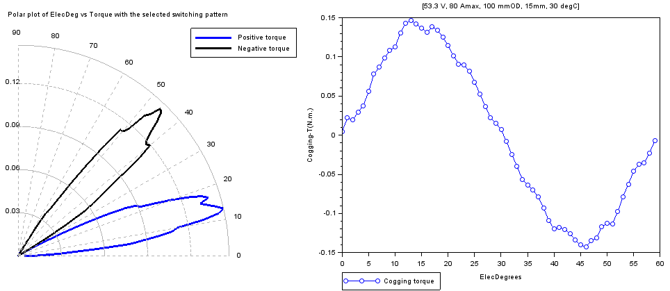
Cogging torque vs rotor angle

char=r1_findMotorChar(Motor,'c')

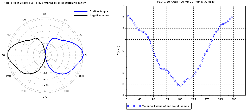
Torque vs rotor angle

With single switch combo turned-on as the rotor rotates for 1 electrical revolution

char=r1_findMotorChar(Motor,'m')

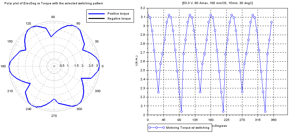
With appropriate switch combo turned-on as the rotor rotates for 1 electrical revolution

char=r1_findMotorChar(Motor,'m_sw')

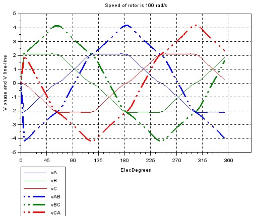
Induced voltages vs rotor angle

char=r1_findMotorChar(Motor,'g')

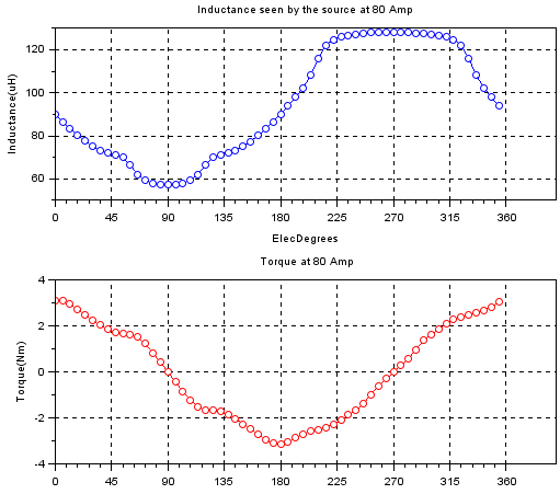
Line inductance & Torque vs Rotor angle

char=r1_findMotorChar(Motor,'ind_sw')

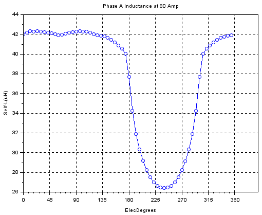
Phase inductance vs Rotor angle

char=r1_findMotorChar(Motor,'ind_A')

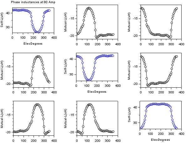
Self and Mutual inductances vs rotor angle

char=r1_findMotorChar(Motor,'ind')

(Torque and Inductance) vs Current Vs rotor position

char=r1_findMotorChar(Motor,'ind_sw_vs_i')

Some animations from the 3d plot resulting from the characterization is presented below.

Radial pull

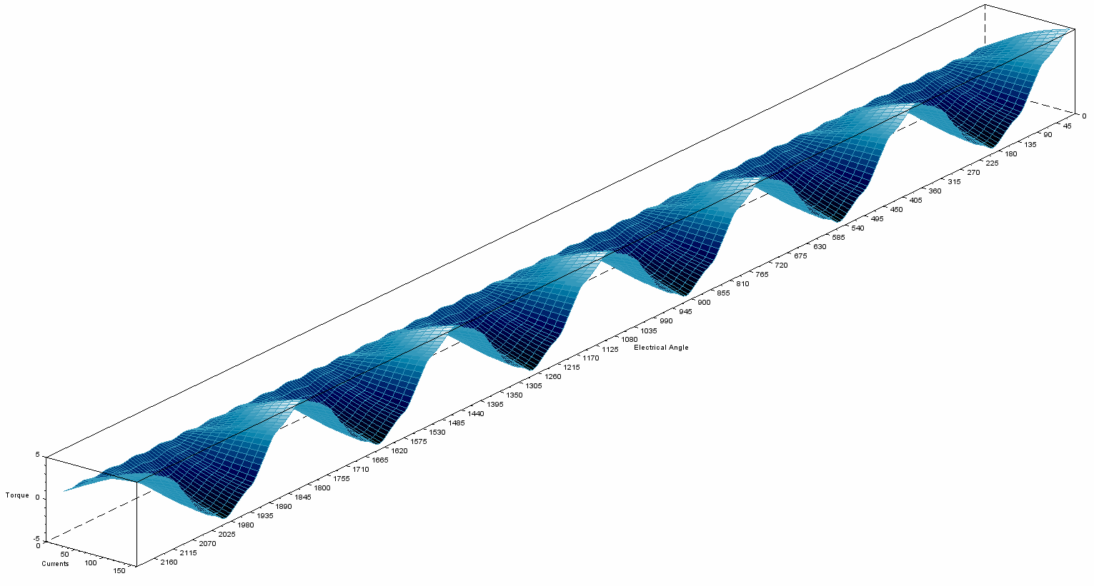
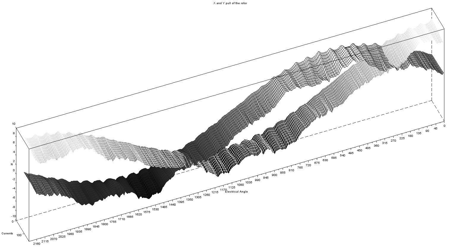
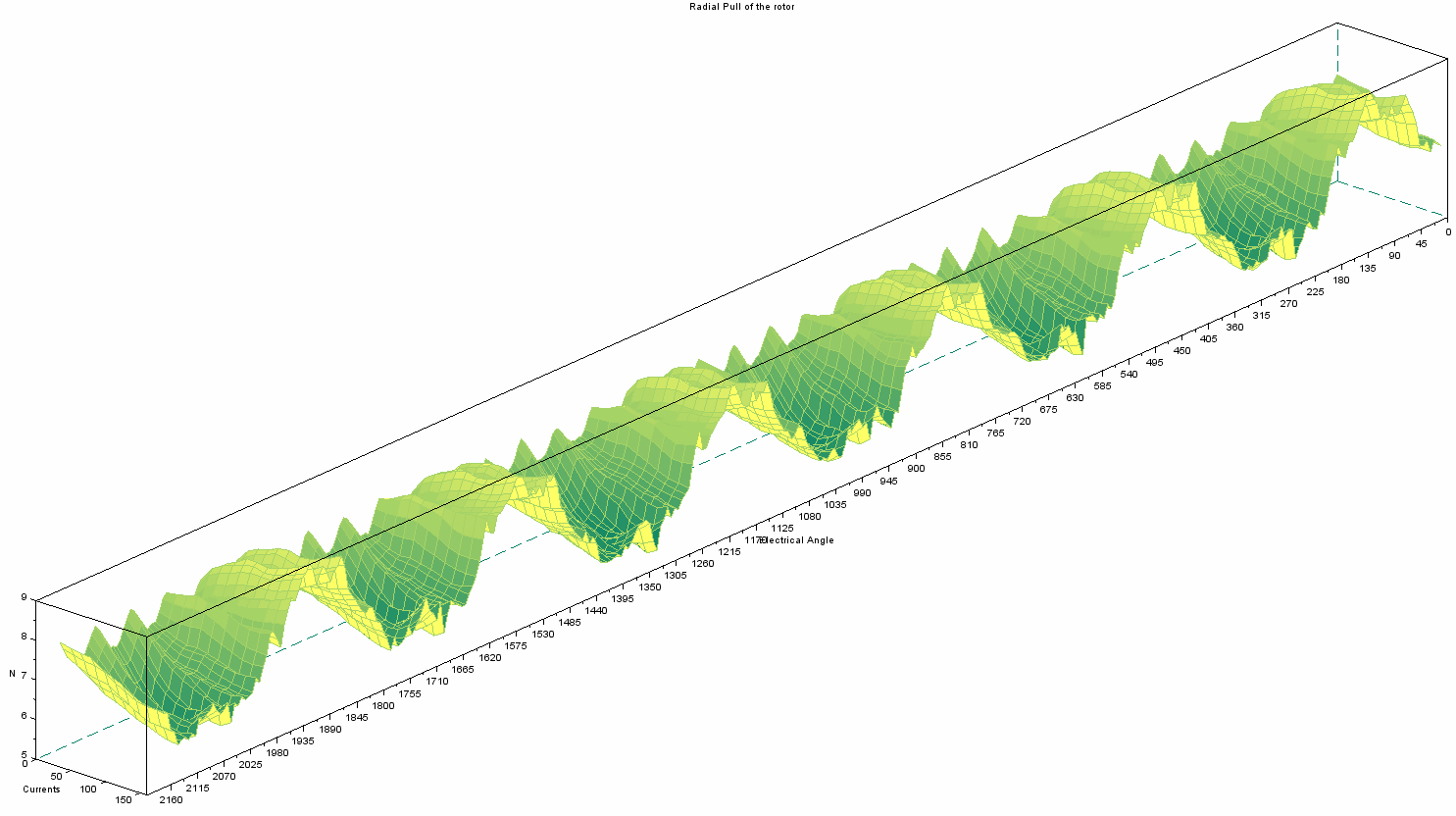
char=r1_findMotorChar(Motor,'m_vs_i')
char=r1_findMotorChar(Motor,'m_vs_i',150,0,11,6)

This characterization gives torque-spread, in addition to the radial pull. The above characterization with a radial offset error of 0.2mm in x direction is run for 6 electrical revolutions (one full mechanical revolution) to give full view of the radial force as below.

Optimization

Initialization

All the optimization related configurations can be stored in a single variable. Default variable can be created from the following script. Every optimization execution happens in its own sandbox environment, undisturbed by the temporary variables or temporary files. Parallel Scilab sessions ( or even scilab console windows) can be run as many as the PC/workstation supports.

opti=r_buildVAR(Motor)
opti=r_buildVAR(0) // or any number, other than motor variable.

When the motor variable is provided, the optimization variable includes the provided variable. When a number is provided, the optimization variable includes the default template of the motor. The following has the motor variable, embedded inside opti variable.

opti.Motor

Methodology

Motor design optimization within the constraints are multivariate optimization problems. Additionally, changing some parameters will also affect the other parameters and/or their boundaries. The optimization technique used for rlib is based on ‘random walk optimization’. All the parameters set to change are changed at every possibility of creating a new model, and whenever a model satisfying the constraints better is found, it is assigned as seed model for the next generation. This is sort of an gradient descent approach, but on a multi-dimensional space.

The optimization has the primary target to maximize the torque. The thresholds for Torque and cornerrpm or nlrpm need to be used to set the lower bounds on the requirements. A Torque threshold of about 1Nm may be set to eliminate all the designs with very low peak torque but very high no load rpm. A cornerrpm or nlrpm of about 100 may be set to eliminate all the designs that may be with zero cornerrpm, or have very low constant-torque-band. The SoC of the motor bay be adjusted to run the optimization for worst voltage conditions, say at 10% SoC. The winding temperature may be adjusted to higher than room temperature, say at 80 degC, to account for increased coil temperature while the motor is in continuous operation. With the worst case conditions set, the optimization is set to result in a better selection of designs.

Settings

Samples

The following sets the number of samples to test before concluding the optimization. The run may be stopped in the middle if needed to.

opti.SampleSize=10000 // usually set to large number so as not to become a limiting factor. 

Change from past value

The following sets the percentage change of the parameters' value based on the conditions specified in ‘Limits’.

opti.PercentChangeInit=25 // set to a number less than 100. Larger number results in drastic variations

When the optimization run is not able to find any better model than the current one even after a lot of trials, the percentage change is set to increase so that the spread of search can be increased. The following variable decides the spread by multiplying the percentagechange with (1+ftchangepct).

opti.frChangePct=0.5 // multiplies PercentChangeInit with 1+frChangePct
opti.NotBetterCountMax=100 // the threshold iterations after which the above operation variable is used 

Tweaking for improvements

The following variable fills the slot with the maximum possible number of turns when the winding turns are to be changed.

opti.getPossibleTurns=1

The following variable uses the better model as the seed model, and proceeds from that model. Without this, the model is just perturbed, and is useful for dimensional tolerance analysis.

opti.DeriveFromLastBest=1

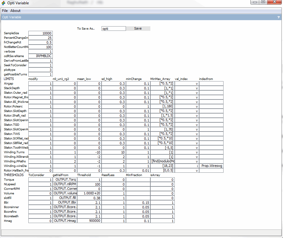
Thresholds

opti.Thresholds

The optimization pass criteria are given using this table. Some important output numbers are provided with thresholds. Only if a given model passes the threshold condition, the model will be saved as odR file and populated in the corresponding plot.

Thresholds are given as numbers, with ‘passifless’ flag. If it is 1, then the threshold inequality changes to ‘<=’, else the inequality stands as ‘>=’. If the value considered is not a single value but rather an array, the ‘MinFraction’ gives an indication of what minimum fraction of the array values need to pass the threshold criteria. The ‘isArray’ field just confirms that this output is an array.

Limits

opti.Limits

The motor parameters that may need to be changed are included in this table.

Setting the modify to 1 results in that parameter changed during optimization.

The n0_un1_rg2 is an important selection for normal distribution, uniform distribution and range. For a normal distribution, mean_low is taken as mean, and the sd_high is taken as standard deviation. For the uniform distribution, mean_low is taken as low boundary, and the sd_high is taken as the high boundary. For the range selection, minmax_array is used for selecting values from the population.

mean_low is mean for standard didsribution(if zero, variable is changed from present value, if non-zero, variable is assigned a value as the computed new value changed from mean), low for uniform distrubution(if min-max array is given only with min and is assigned -100, a random value is assigned to the variable from the low and high), NA for range.

sd_high is standard deviation for normal dsitrubution(if zero, sd is computed from min_max array bounds {min-max} /6. still depends on mean for offset from present or assign as new), high for a uniform distrubution, NA for range

The minChange is an important parameter to include the process parameters, i.e. the minimum change in the geometry. For example, the number of turns can not be changed from 1 to 1.1. It has to be either 2 or 3.

The minmax_array is used as the boundary values for the parameters after they are passed through the distribution. This value can be either a no value [] (no bounds), or single value ( min only) or two values( min and max values). Each value can be an integer itself indicating an absolute value, or a value followed by a star symbol, indicating a multiplication with the present value of the parameter.

The val_index is to indicate whether the final output is a direct value or an input to the array as an index. V is to say that the value is updatd to the parameter as it is obtained, and i is to say that the obtained value is used as an index to obtain the updated parameter’s value from the indexfrom field.

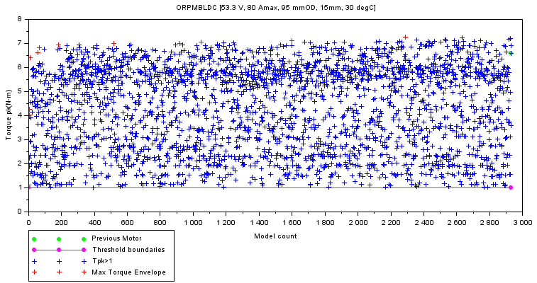
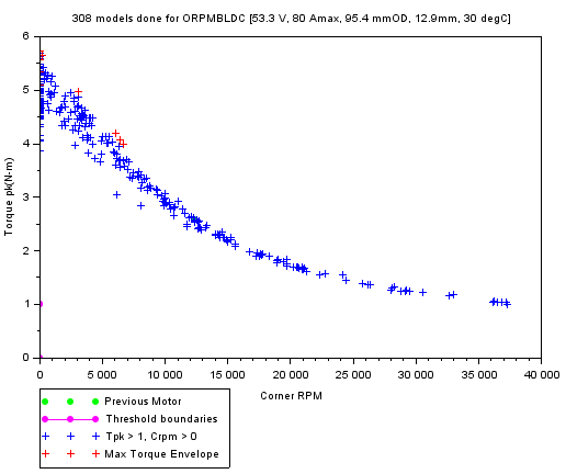
Plots from optimization

The plots can be chosen to be either Torque-ModelCount or Torque-CornerRPM or Torque-MaxRPM. Essentially these are different representations of the same data. Since the optimization plots look similar irrespective of the geometry, I have presented the same images from the ORBLDC model’s optimization run.

Data

Handling the Data

Motor model data is saved in .odR files ( odR stands for Optimization Data Record) and the optimization settings data is saved in .osR files (osR stands for Optimization Settings Record).

Save the model

filename=r1_saveRecord(Motor,'myMotorName','extraString')
filename=r1_saveRecord(opti,'myOptiSetting','extraString')

This function requires an optimization or Motor structure and the name of the variable to be stored in .osR/.odR as the optimization/Motor variable. This function returns the filename.

Script to save the model’s variable

r1_saveRecord(Motor,'testMotorName')

This saves the variable Motor in the file titled testMotorName_20171014111055.odR, where the number string represents the date and time of saving the variable.

Load the model

Motor=r_loadRecord('.\1.odR')
opti=r_loadRecord('.\1.osR')

This function loads the optimization/Motor structure from the osR file. If the file has an optimization settings record, optimization structure’s Motor field needs to be updated with your own Motor structure. Add optional second argument ‘preserve’ if you want to preserve the original fields from the file.

Script to load the individual motor variable from the saved file is below.

Motor=r_loadRecord('testMotorName_20171014111055.odR')

odr2csv

After an optimization run, many odR files get accumulated. Reading individual files to get their contents and comparing individual files is difficult, and impractical. The following function reads all the odR files in the present working directory and stores all of their contents in a csv (comma separated variables) file. This file can later be used to sort and filter based on the requirement.

r_odR2csv('Y:\MOTOR\scripts\r_lib\r_common_odr.bin',50,'par')
r_odR2csv('Y:\MOTOR\scripts\r_lib\r_common_odr.bin','par')
r_odR2csv('Y:\MOTOR\scripts\r_lib\r_common_odr.bin')

This function can be used as a standalone scilab mode, or a parallel scilab mode. In standalone mode, as indicated by the lack of ‘par’ keyword in the function call, present scilab session reads each odR file in sequence and updates the csv file.

With the ‘par’ keyword, multiple parallel Scilab sessions are started in the background, each operating on a set of individual odR files, the number may be specified or not. If the number is not specified, 50 is taken as default. This par method is most effective if the number of odR files to read is more.

This function requires the path of compiled function file(*.bin) which has this function. Most likely it will be r_common_odr.bin. Each background session is expected to occupy 200MB to 250MB. Carefully choose the parallel sessions to leave enough space for other programs on the PC. If you have 12GB RAM installed, 7GB still un-utilized as seen from the Windows task manager, then use 5GB (about 70 percent) for scilab, i.e. you can run 20 scilab sessions, max. If you have N odR files, then call odr2csv (lib , N/20 , par). If the N/20 becomes more than 500, consider that each scilab takes more memory. It becomes iterative. Instead, use the feature without par, plain old way.

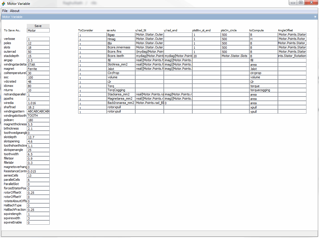
GUI

Motor

All the script based operations to change the motor parameters, and saving the model from command prompt can be done from the GUI too. The settings can be saved using the save button. Don’t use space or numbers at the beginning of the string for the name.

Optimization

All the script based operations to change the optimization parameters, and saving the settings from command prompt can be done from the GUI too. The settings can be saved using the save button. Don’t use space or numbers at the beginning of the string for the name.